




ElasticSearch 入门:查询与聚合基础使用指南
一、准备工作:导入示例数据
以 Elasticsearch 官方推荐的 NYC 黄色出租车数据 为例,通过以下步骤导入数据:
1. 创建索引并导入数据
在 Kibana 的 Dev Tools 中执行批量导入(Bulk API):
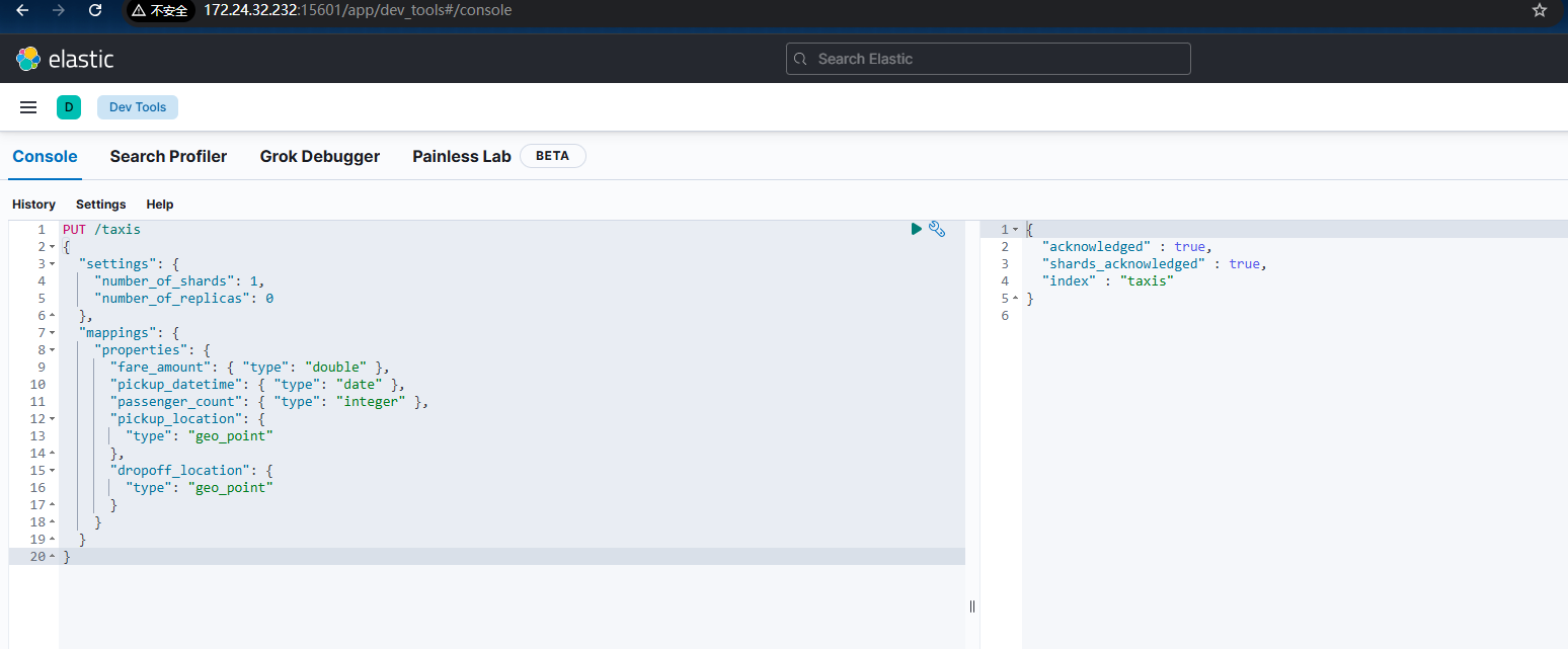
// 创建索引
PUT /taxis
{
  "settings": {
    "number_of_shards": 1,
    "number_of_replicas": 0
  },
  "mappings": {
    "properties": {
      "fare_amount": { "type": "double" },
      "passenger_count": { "type": "integer" },
      "pickup_location": {
        "type": "geo_point"
      },
      "dropoff_location": {
        "type": "geo_point"
      },
       "pickup_datetime": {
        "type": "date",
        "format": "yyyy-MM-dd HH:mm:ss||strict_date_optional_time||epoch_millis"
      }
    }
  }
}


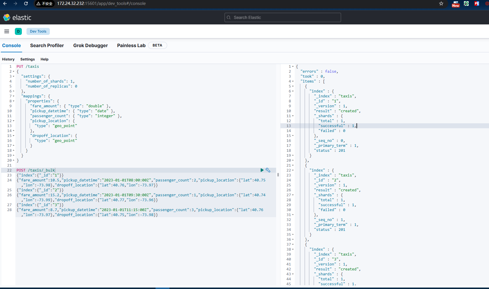
// 批量导入数据(示例数据需从GitHub获取,此处为简化格式)
POST /taxis/_bulk
{"index":{"_id":"1"}}
{"fare_amount": 10.5, "pickup_datetime": "2023-01-01 08:00:00", "passenger_count": 2, "pickup_location": {"lat": 40.75, "lon": -73.98}, "dropoff_location": {"lat": 40.76, "lon": -73.97}}
{"index":{"_id":"2"}}
{"fare_amount": 15.2, "pickup_datetime": "2023-01-01 09:30:00", "passenger_count": 1, "pickup_location": {"lat": 40.74, "lon": -73.99}, "dropoff_location": {"lat": 40.77, "lon": -73.96}}
{"index":{"_id":"3"}}
{"fare_amount": 8.7, "pickup_datetime": "2023-01-01 11:15:00", "passenger_count": 3, "pickup_location": {"lat": 40.76, "lon": -73.97}, "dropoff_location": {"lat": 40.75, "lon": -73.98}}
// 更多数据...
2. 确认数据导入成功
导入更多数据示例
POST /taxis/_bulk
{"index":{"_id":"4"}}
{"fare_amount":12.3,"pickup_datetime":"2023-01-01 13:45:00","passenger_count":1,"pickup_location":{"lat":40.73,"lon":-73.99},"dropoff_location":{"lat":40.78,"lon":-73.95}}
{"index":{"_id":"5"}}
{"fare_amount":9.8,"pickup_datetime":"2023-01-01 14:20:00","passenger_count":2,"pickup_location":{"lat":40.75,"lon":-74.01},"dropoff_location":{"lat":40.74,"lon":-73.98}}
{"index":{"_id":"6"}}
{"fare_amount":18.5,"pickup_datetime":"2023-01-01 15:10:00","passenger_count":3,"pickup_location":{"lat":40.72,"lon":-73.98},"dropoff_location":{"lat":40.79,"lon":-73.93}}
{"index":{"_id":"7"}}
{"fare_amount":7.2,"pickup_datetime":"2023-01-01 16:30:00","passenger_count":1,"pickup_location":{"lat":40.76,"lon":-73.96},"dropoff_location":{"lat":40.75,"lon":-73.99}}
{"index":{"_id":"8"}}
{"fare_amount":14.6,"pickup_datetime":"2023-01-01 17:45:00","passenger_count":4,"pickup_location":{"lat":40.71,"lon":-73.97},"dropoff_location":{"lat":40.80,"lon":-73.92}}
{"index":{"_id":"9"}}
{"fare_amount":11.3,"pickup_datetime":"2023-01-01 18:15:00","passenger_count":2,"pickup_location":{"lat":40.74,"lon":-74.00},"dropoff_location":{"lat":40.75,"lon":-73.97}}
{"index":{"_id":"10"}}
{"fare_amount":16.7,"pickup_datetime":"2023-01-01 19:20:00","passenger_count":3,"pickup_location":{"lat":40.70,"lon":-73.96},"dropoff_location":{"lat":40.81,"lon":-73.91}}
{"index":{"_id":"11"}}
{"fare_amount":8.9,"pickup_datetime":"2023-01-01 20:30:00","passenger_count":1,"pickup_location":{"lat":40.77,"lon":-73.95},"dropoff_location":{"lat":40.73,"lon":-74.00}}
{"index":{"_id":"12"}}
{"fare_amount":13.4,"pickup_datetime":"2023-01-01 21:45:00","passenger_count":2,"pickup_location":{"lat":40.69,"lon":-73.95},"dropoff_location":{"lat":40.82,"lon":-73.90}}
{"index":{"_id":"13"}}
{"fare_amount":19.2,"pickup_datetime":"2023-01-01 22:10:00","passenger_count":4,"pickup_location":{"lat":40.73,"lon":-74.02},"dropoff_location":{"lat":40.72,"lon":-73.97}}
{"index":{"_id":"14"}}
{"fare_amount":6.5,"pickup_datetime":"2023-01-01 23:30:00","passenger_count":1,"pickup_location":{"lat":40.78,"lon":-73.94},"dropoff_location":{"lat":40.72,"lon":-73.99}}
{"index":{"_id":"15"}}
{"fare_amount":15.8,"pickup_datetime":"2023-01-02 00:15:00","passenger_count":2,"pickup_location":{"lat":40.68,"lon":-73.94},"dropoff_location":{"lat":40.83,"lon":-73.89}}
{"index":{"_id":"16"}}
{"fare_amount":10.3,"pickup_datetime":"2023-01-02 01:45:00","passenger_count":1,"pickup_location":{"lat":40.75,"lon":-74.01},"dropoff_location":{"lat":40.73,"lon":-73.98}}
{"index":{"_id":"17"}}
{"fare_amount":17.6,"pickup_datetime":"2023-01-02 02:30:00","passenger_count":3,"pickup_location":{"lat":40.67,"lon":-73.93},"dropoff_location":{"lat":40.84,"lon":-73.88}}
{"index":{"_id":"18"}}
{"fare_amount":9.1,"pickup_datetime":"2023-01-02 03:45:00","passenger_count":2,"pickup_location":{"lat":40.76,"lon":-74.00},"dropoff_location":{"lat":40.74,"lon":-73.97}}
{"index":{"_id":"19"}}
{"fare_amount":14.2,"pickup_datetime":"2023-01-02 04:20:00","passenger_count":4,"pickup_location":{"lat":40.66,"lon":-73.92},"dropoff_location":{"lat":40.85,"lon":-73.87}}
{"index":{"_id":"20"}}
{"fare_amount":8.5,"pickup_datetime":"2023-01-02 05:30:00","passenger_count":1,"pickup_location":{"lat":40.77,"lon":-73.99},"dropoff_location":{"lat":40.73,"lon":-73.96}}
{"index":{"_id":"21"}}
{"fare_amount":12.9,"pickup_datetime":"2023-01-02 06:45:00","passenger_count":2,"pickup_location":{"lat":40.65,"lon":-73.91},"dropoff_location":{"lat":40.86,"lon":-73.86}}
{"index":{"_id":"22"}}
{"fare_amount":16.3,"pickup_datetime":"2023-01-02 07:30:00","passenger_count":3,"pickup_location":{"lat":40.74,"lon":-74.03},"dropoff_location":{"lat":40.72,"lon":-73.95}}
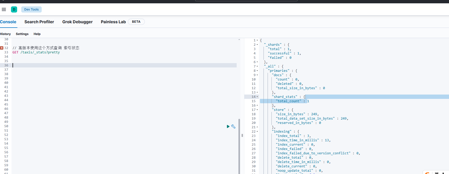
// 查看索引状态
GET /taxis/_status
高版本使用 GET /taxis/_stats?pretty
可以通过 Get / 获取当前版本
// 查看文档总数
GET /taxis/_count
二、基础查询操作
常见查询类型对比
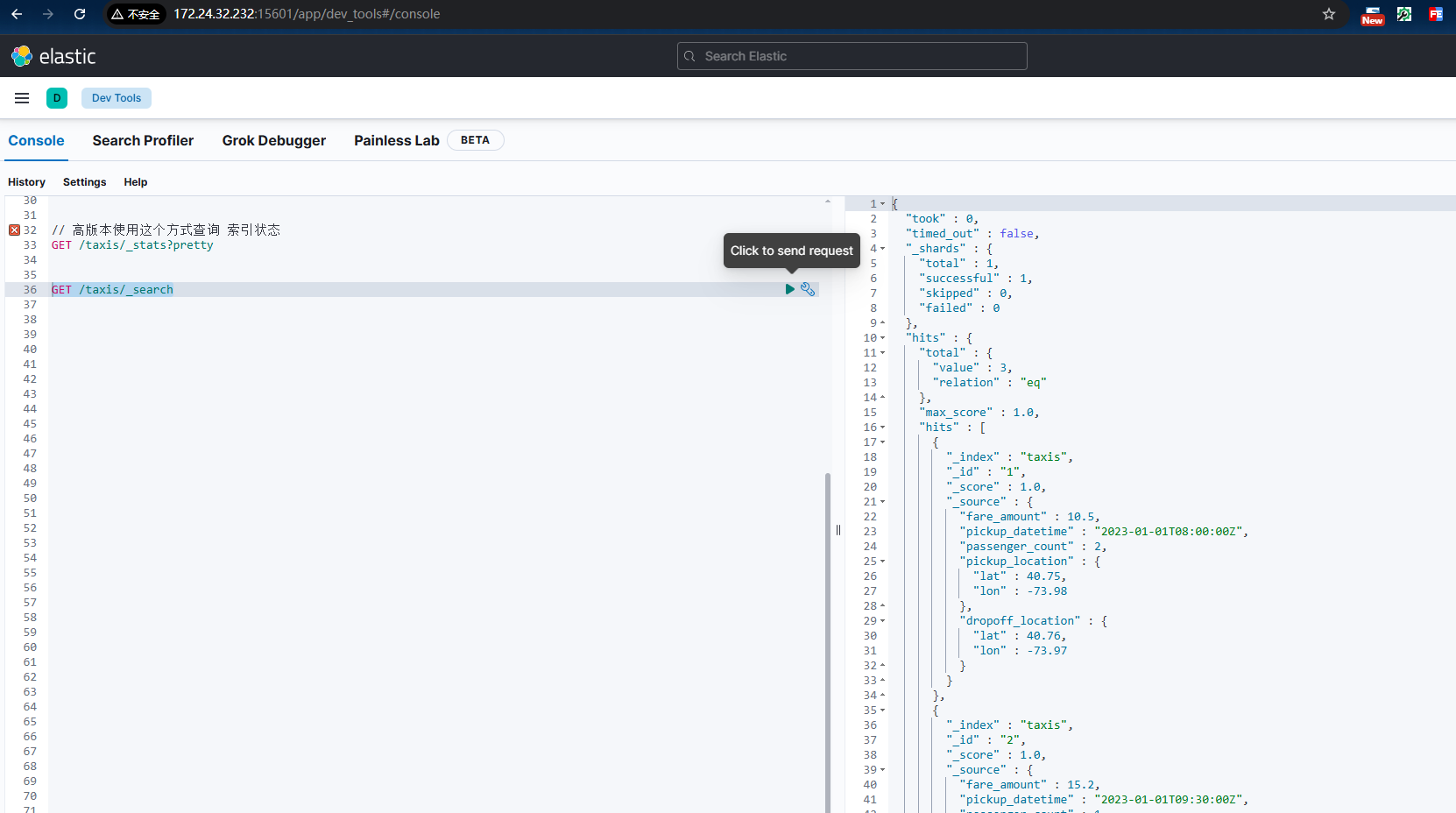
1. 查询所有文档(match_all)
GET /taxis/_search
{
  "query": {
    "match_all": {}
  }
}
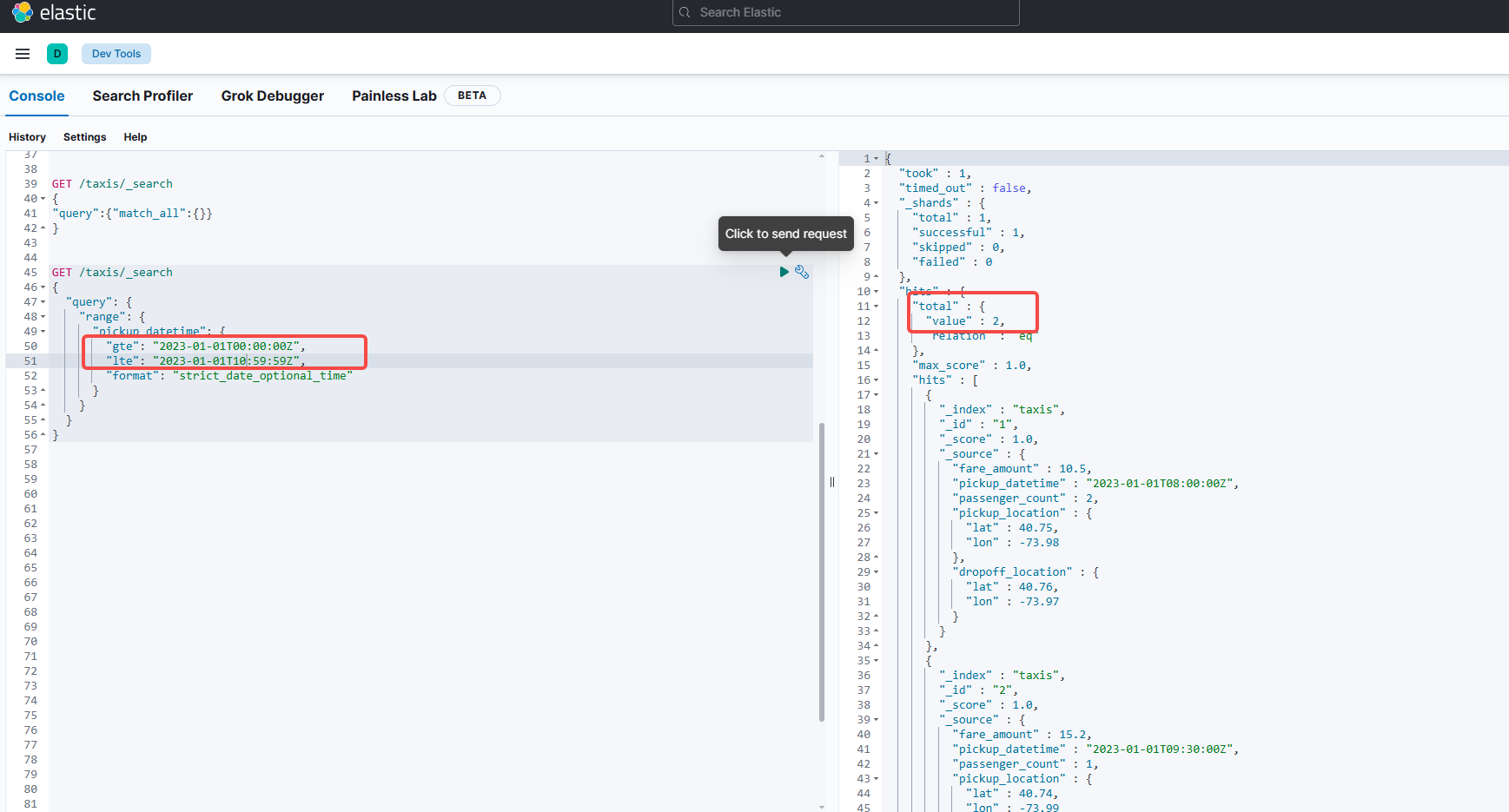
// 查询上午 9 点之后的订单,并按价格降序排列:
GET /taxis/_search
{
  "query": {
    "range": {
      "pickup_datetime": {
        "gte": "2023-01-01T09:00:00Z"
      }
    }
  },
  "sort": [
    {
      "fare_amount": {
        "order": "desc"
      }
    }
  ]
}
说明:返回索引中所有文档,适用于数据量小的场景,大数量级需配合分页。
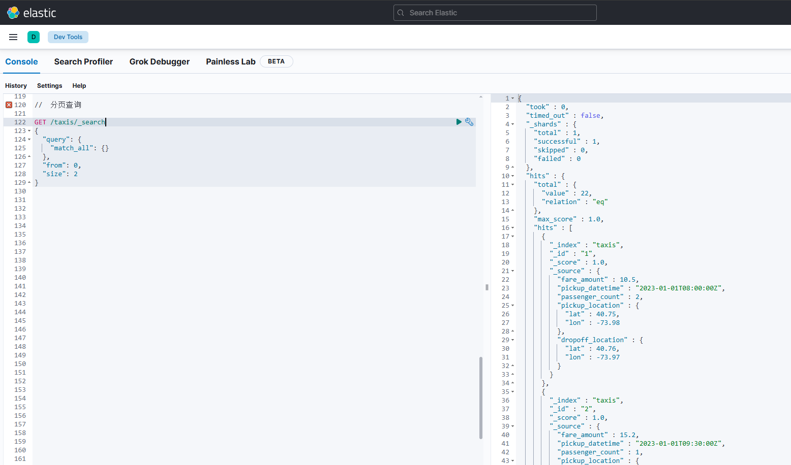
2. 分页查询(from + size)
GET /taxis/_search
{
  "query": {
    "match_all": {}
  },
  "from": 0,  // 起始偏移量
  "size": 2   // 每页显示数量
}
注意:ES 默认分页深度限制为 10000 ,深度分页需使用 Scroll 或 Search After。可以使用PUT /taxis/_settings 修改深度分页大小。深度分页的原理我们后面再聊。
可以使用
PUT /taxis/_settings
{
  "index.max_result_window": 50000
}
3. 指定字段查询(_source)
GET /taxis/_search
{
  "query": {
    "match_all": {}
  },
  "_source": ["fare_amount", "pickup_datetime"]  // 只返回指定字段
}
4. 文本匹配查询(match)
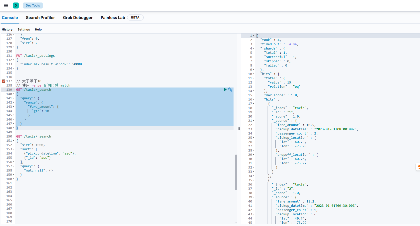
// 查询费用大于10的记录
GET /taxis/_search
{
  "query": {
    "range": {
      "fare_amount": {
        "gte": 10  // 大于等于10
      }
    }
  }
}

// 文本分词匹配(如查询包含"morning"的时间)
GET /taxis/_search
{
  "query": {
    "match": {
      "pickup_datetime": "morning"
    }
  }
}

GET /taxis/_search
{
  "size": 1000,
  "sort": [
    {"pickup_datetime": "asc"},  // 必须包含至少一个唯一排序字段
    {"_id": "asc"}
  ],
  "query": {
    "match_all": {}
  }
}
5. 短语匹配查询(match_phrase)
// 精确匹配短语(分词顺序必须一致)
GET /taxis/_search
{
  "query": {
    "match_phrase": {
      "pickup_location.lat": "40.75"
    }
  }
}
6. 多条件组合查询(bool)
// 查询费用大于10且乘客数为2的记录
GET /taxis/_search
{
  "query": {
    "bool": {
      "must": [  // 必须同时满足
        { "match": { "fare_amount": { "gte": 10 } } },
        { "match": { "passenger_count": 2 } }
      ]
    }
  }
}

// 查询费用大于10或乘客数大于2的记录
GET /taxis/_search
{
  "query": {
    "bool": {
      "should": [  // 满足任意一个
        { "match": { "fare_amount": { "gte": 10 } } },
        { "match": { "passenger_count": { "gt": 2 } } }
      ]
    }
  }
}

// 查询费用大于10但排除乘客数为1的记录
GET /taxis/_search
{
  "query": {
    "bool": {
      "must": [
        { "match": { "fare_amount": { "gte": 10 } } }
      ],
      "must_not": [  // 必须不满足
        { "match": { "passenger_count": 1 } }
      ]
    }
  }
}
7. 过滤查询(filter)
// 高效过滤(不计算分数,可缓存)
GET /taxis/_search
{
  "query": {
    "bool": {
      "filter": [
        { "range": { "fare_amount": { "gte": 10, "lte": 20 } } },
        { "term": { "passenger_count": 2 } }
      ]
    }
  }
}
对地理坐标使用专用查询:
geo_bounding_box:矩形区域查询geo_distance:距离中心点一定范围内的查询geo_polygon:多边形区域查询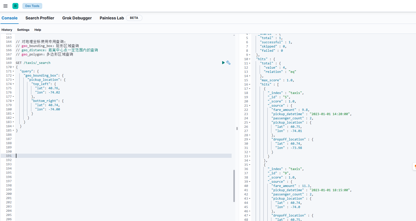
三、聚合查询(Aggregation)基础
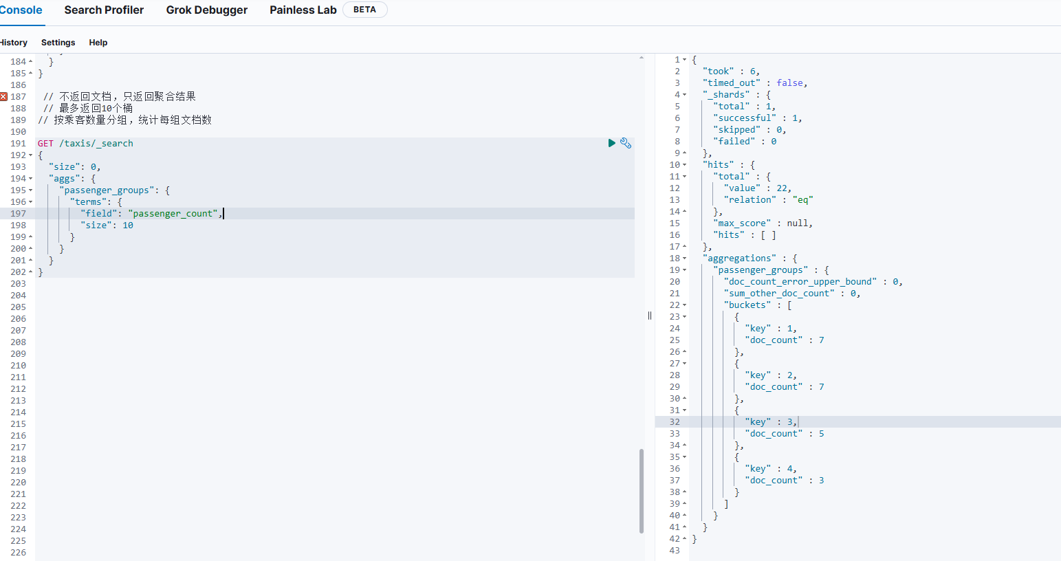
1. 简单桶聚合(Terms)
按乘客数量分组,统计每组文档数
// 按乘客数量分组,统计每组文档数
GET /taxis/_search
{
  "size": 0,  // 不返回文档,只返回聚合结果
  "aggs": {
    "passenger_groups": {
      "terms": {
        "field": "passenger_count",
        "size": 10  // 最多返回10个桶
      }
    }
  }
}
2. 指标聚合(Metrics)
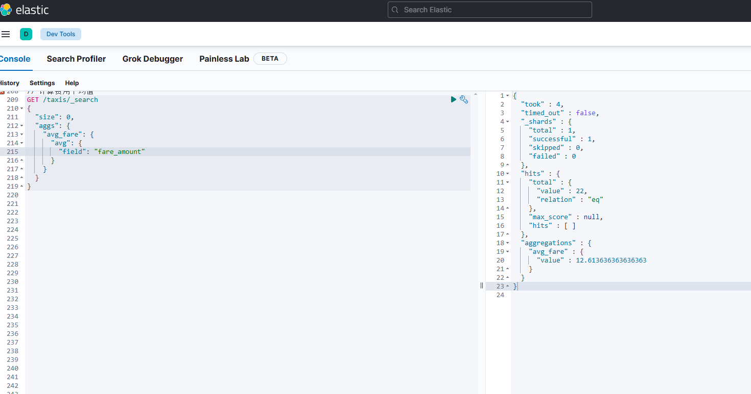
计算费用平均值
计算费用总和与最大值
// 计算费用平均值
GET /taxis/_search
{
  "size": 0,
  "aggs": {
    "avg_fare": {
      "avg": {
        "field": "fare_amount"
      }
    }
  }
}

// 计算费用总和与最大值
GET /taxis/_search
{
  "size": 0,
  "aggs": {
    "fare_stats": {
      "stats": {  // 一次性获取多种指标
        "field": "fare_amount"
      }
    }
  }
}
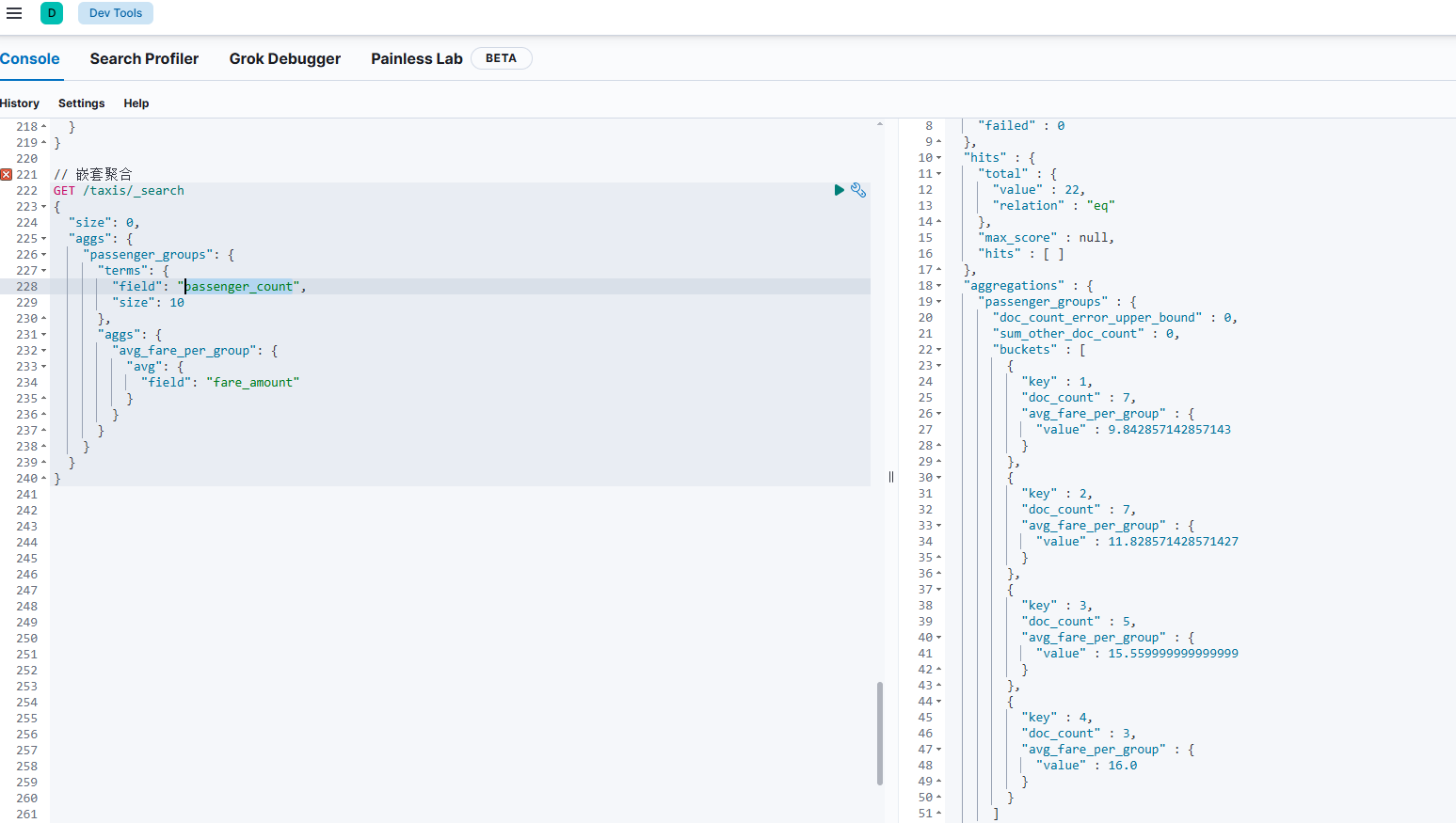
3. 嵌套聚合(Bucket + Metric)
GET /taxis/_search
{
  "size": 0,  // 不返回原始文档,只返回聚合结果
  "aggs": {  // 定义聚合操作
    "passenger_groups": {  // 自定义聚合名称:按乘客数量分组
      "terms": {  // 分组类型:按字段值分组
        "field": "passenger_count",  // 按乘客数量字段分组
        "size": 10  // 最多返回10个分组(默认按文档数降序排列)
      },
      "aggs": {  // 嵌套聚合:在每个分组内进行二次聚合
        "avg_fare_per_group": {  // 自定义聚合名称:计算平均费用
          "avg": {  // 聚合类型:平均值
            "field": "fare_amount"  // 对费用字段计算平均值
          }
        }
      }
    }
  }
}
4. 地理距离聚合(Geo Distance)
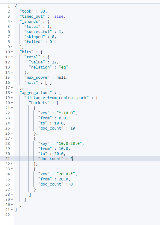
地理距离聚合(geo_distance) 功能,用于分析出租车订单的上车地点(pickup_location)与中央公园(坐标:40.7649, -73.9731)的距离分布情况。让我拆解它的具体含义:
查询功能
GET /taxis/_search
{
  "size": 0,  // 不返回原始文档,只返回聚合结果
  "aggs": {  // 定义聚合操作
    "distance_from_central_park": {  // 聚合名称:距离中央公园的分布
      "geo_distance": {  // 地理距离聚合类型
        "field": "pickup_location",  // 地理坐标字段(上车地点)
        "origin": { "lat": 40.7649, "lon": -73.9731 },  // 中心点:中央公园
        "unit": "km",  // 距离单位:公里
        "ranges": [  // 定义距离区间
          { "to": 10 },  // 0-10公里
          { "from": 10, "to": 20 },  // 10-20公里
          { "from": 20 }  // 20公里以上
        ]
      }
    }
  }
}
5. 对聚合结果排序
// 按平均费用降序排列分组结果
GET /taxis/_search
{
  "size": 0,
  "aggs": {
    "passenger_groups": {
      "terms": {
        "field": "passenger_count",
        "size": 10,
        "order": {  // 排序规则
          "avg_fare_per_group": "desc"  // 按嵌套聚合结果排序
        }
      },
      "aggs": {
        "avg_fare_per_group": {
          "avg": {
            "field": "fare_amount"
          }
        }
      }
    }
  }
}
四、Kibana 可视化操作
创建仪表盘:
进入 Kibana → Dashboard → Create dashboard
添加可视化组件,如按乘客数量分组的柱状图(使用Terms聚合)。
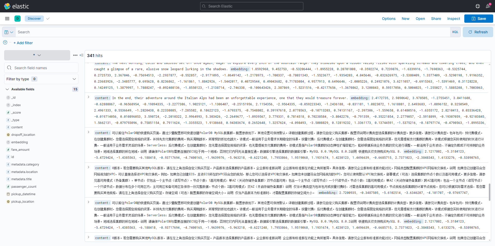
使用Discover面板查询:
进入 Kibana → Discover → 选择索引
taxis通过图形界面构建查询条件,实时查看结果。
五、进阶提示
查询性能优化:
优先使用
filter而非query,提升查询效率。对频繁查询的字段创建索引(如
fare_amount)。
聚合深度限制:
大桶聚合(如Terms)需设置
shard_size参数,避免内存溢出。
查询性能优化指南
你提到的两点建议非常正确,下面我将详细展开这两种优化方法,并提供具体实现示例:
一、优先使用Filter而非Query
1. 核心原理
Query上下文:计算文档与查询的匹配度评分(_score),适用于全文搜索
Filter上下文:只判断文档是否匹配,不计算评分,结果会被缓存,适合频繁使用的过滤条件
2. 优化示例
原查询(使用query)
GET /taxis/_search
{
  "query": {
    "bool": {
      "must": [
        {"match": {"passenger_count": 2}},
        {"range": {"fare_amount": {"gte": 10}}}
      ]
    }
  }
}
优化后(使用filter)
GET /taxis/_search
{
  "query": {
    "bool": {
      "filter": [  // 使用filter替代must
        {"term": {"passenger_count": 2}},  // 精确匹配用term
        {"range": {"fare_amount": {"gte": 10}}}
      ]
    }
  }
}
3. 性能对比
缓存机制:filter结果会被缓存,相同条件重复查询时直接使用缓存
执行效率:filter跳过评分计算,内存和CPU开销更小
二、对频繁查询的字段创建索引
1. 检查现有映射
GET /taxis/_mapping2. 为数值字段添加doc_values(默认已启用)
PUT /taxis/_mapping
{
  "properties": {
    "fare_amount": {
      "type": "double",
      "doc_values": true  // 用于快速过滤和聚合
    },
    "passenger_count": {
      "type": "integer",
      "doc_values": true
    }
  }
}
3. 为文本字段指定合适的分词器
PUT /taxis/_mapping
{
  "properties": {
    "payment_type": {  // 假设存在支付类型字段
      "type": "keyword"  // 不分词,用于精确匹配
    }
  }
}
4. 地理位置字段优化
PUT /taxis/_mapping
{
  "properties": {
    "pickup_location": {
      "type": "geo_point",
      "fields": {
        "hash": {  // 添加geohash子字段
          "type": "geo_point",
          "geohash_precision": "1km"  // 精度为1公里
        }
      }
    }
  }
}
三、其他性能优化技巧
1. 聚合查询优化
原聚合(未优化)
GET /taxis/_search
{
  "size": 0,
  "aggs": {
    "fare_ranges": {
      "range": {
        "field": "fare_amount",
        "ranges": [
          {"to": 10},
          {"from": 10, "to": 20},
          {"from": 20}
        ]
      }
    }
  }
}
优化后(添加全局过滤)
GET /taxis/_search
{
  "size": 0,
  "query": {
    "bool": {
      "filter": [
        {"range": {"pickup_datetime": {"gte": "2023-01-01"}}}
      ]
    }
  },
  "aggs": {
    "fare_ranges": {
      "filter": {
        "term": {"payment_type": "credit_card"}  // 只统计信用卡支付
      },
      "aggs": {
        "range": {
          "field": "fare_amount",
          "ranges": [...]
        }
      }
    }
  }
}
2. 分页查询优化
深度分页问题
GET /taxis/_search
{
  "from": 9000,
  "size": 100
}
优化方案(使用search_after)
GET /taxis/_search
{
  "size": 100,
  "sort": [
    {"pickup_datetime": "desc"},
    {"_id": "desc"}
  ],
  "search_after": [1672531200000, "100"]  // 从上一页最后一条记录继续
}
3. 索引设置优化
PUT /taxis/_settings
{
  "index.refresh_interval": "30s",  // 降低刷新频率,提高写入性能
  "index.number_of_replicas": 1,    // 生产环境通常设置为1
  "index.blocks.read_only_allow_delete": false  // 确保索引可写
}
四、性能监控与分析
使用Explain API分析查询执行计划
GET /taxis/_explain/1
{
  "query": {
    "range": {"fare_amount": {"gte": 15}}
  }
}
查看慢查询日志
# elasticsearch.yml配置
index.search.slowlog.threshold.query.warn: 10s
index.search.slowlog.threshold.fetch.warn: 5s
使用Profile API分析查询性能
GET /taxis/_search?profile=true
{
  "query": {
    "bool": {
      "filter": [
        {"term": {"passenger_count": 2}},
        {"range": {"fare_amount": {"gte": 10}}}
      ]
    }
  }
}
通过上述优化措施,通常可以将查询性能提升数倍到数十倍,具体效果取决于数据规模和查询复杂度。建议在生产环境前进行基准测试,对比优化前后的性能差异。
官方文档参考:
评论区